Students sometimes feel that linear approximations and Taylor polynomials are an unnecessary mathematical excursion. After all, the examples used to illustrate the ideas usually start with some function f(x) and then proceed to obtain an approximation to this function that is useful only for some restricted set of values of x. So they rightly ask, “if we already have the function f(x), why on earth would we ever want an approximation to this function that works only for restricted values of x?” There are at least two answers to this question.
First, if the function f(x) is to be used in further calculations and derivations then this can sometimes be difficult (or even impossible) if f(x) is complicated. In such cases we might be willing to settle for an approximation to f(x) if this means that we can conduct further analyses.
Second, in many instances we will not actually have an expression for the function f(x). Perhaps surprisingly though, we can still sometimes obtain a Taylor polynomial approximation to this function. This is because, even though we might not know the function f(x), we might still be able to calculate its derivatives at a point of interest. And knowing the derivatives of f(x) at a point x = a is all that is required to construct the Taylor polynomial for the function at this point. The Project in Section 3.8 of the textbook illustrates this idea. The material below explores the project in more depth.
The following animation allows you to explore the Ricker difference equation model for the harvesting of renewable resources. The initial population size is fixed at 1 and the remaining constants can be varied continuously using the sliders.
The black curve below shows the limiting population size as time t gets large for the Ricker model, as a function of the harvesting rate h. This curve was obtained numerically using a CAS because it is not possible to obtain an explicit expression for this function. Notice that the limiting population size drops discontinuously to zero as the harvest rate h increases past approximately h = 0.72. The blue line is the first order Taylor polynomial approximation that you will derive in Problem 4 of this project. The green curve is the second-order Taylor polynomial approximation that you will derive in Problem 5 of this project.
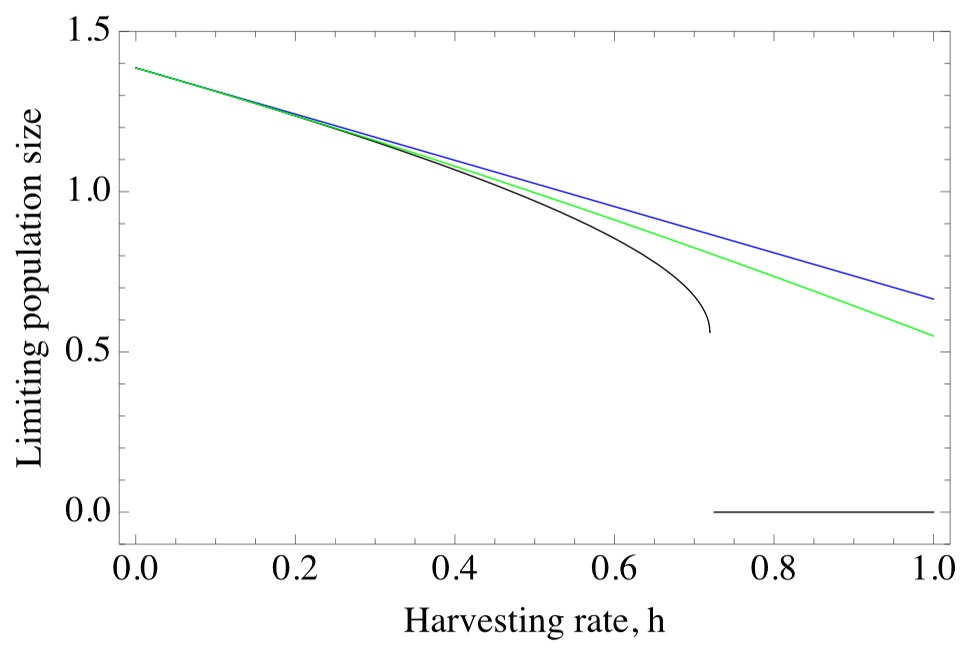
These results demonstrate that, even though we cannot derive the function giving the limiting population size, we can nevertheless derive approximations to this function using Taylor polynomials. As expected, the second-order Taylor polynomial provides a better approximation than the first-order Taylor polynomial. Both approximations become poor when the harvest rate h is not near zero.