The shape of the relationship between the number of amphibian species and area presented in Example 4.2.5 of the textbook is similar to that of many other groups of organisms. Two additional examples from Africa are presented in Figure 1 below (data can be downloaded from the links at the left).
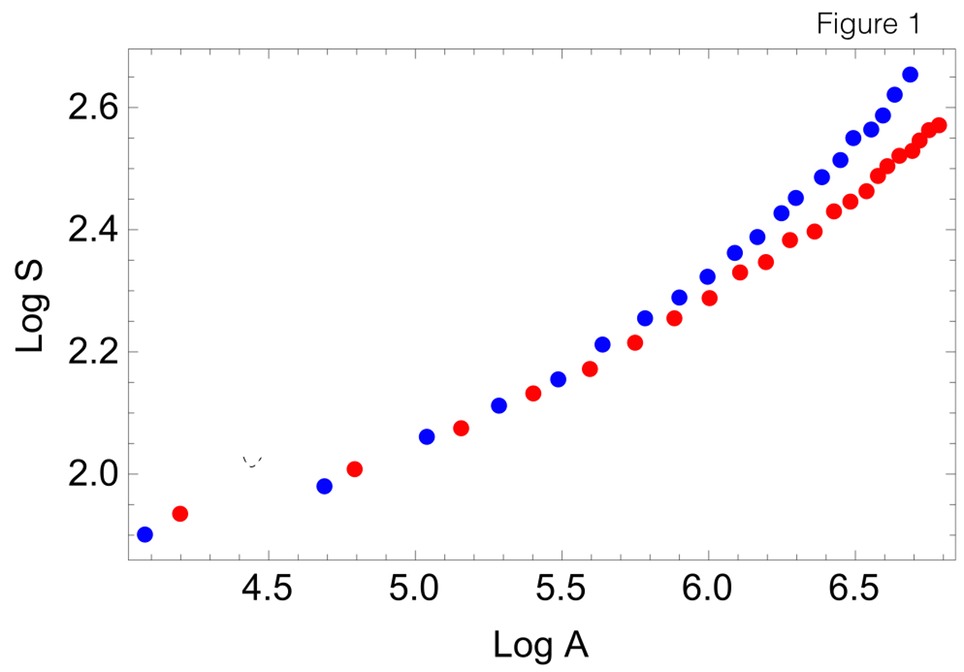
The red dots are measurements for birds and the blue dots are those for mammals. Again you can see that both relationships appear to be concave upward.
To gain a better understanding of the biological significance of this concavity let’s focus on mammals only (the blue dots). To approximate the derivative of the relationship show in Figure 1 at different values of Log A, let’s calculate the slopes of the line segments that connect successive data points (see Figure 2).
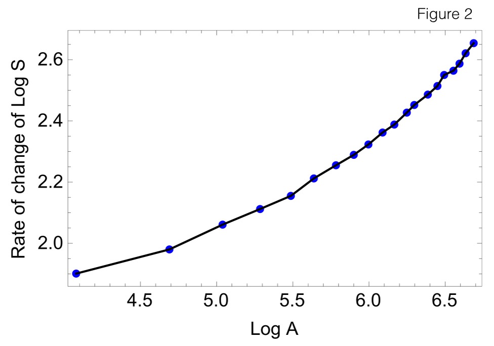
The slope of each line segment in Figure 2 is plotted in Figure 3, as a function of the value of Log A of the left-hand endpoint of the segment.
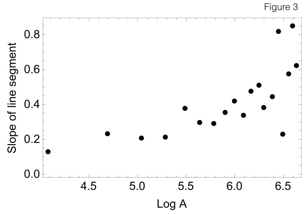
Figure 3 reveals a general trend for the slopes of the line segments in Figure 2 to get bigger (that is, steeper) as the value of Log A increases. This is reflective of the fact that the relationship shown in Figure 1 is concave upward. The slopes of the line segments in Figure 2 represent the increase in the number of species that occurs with an increase in area (both on a log scale). Therefore, Figure 3 shows that this increase in the number of species with area, itself gets larger as area increases. This is precisely what it means for the species-area relationship to be concave upward.
References
Data are from Storch et al. 2012. Universal species-area and endemics-area relationships at continental scales. Nature 488:78-83