Throughout the textbook we have seen different examples of a logistic model. For instance, on Pages 74 and 97 of the textbook we introduced the logistic difference equation for modeling population size (also see Examples 2.1.8 and 4.5.4 and the associated ‘BB' material on this website).
In addition to the discrete-time examples involving the logistic difference equation, we also saw in Example 2.2.8 of the textbook that a continuous-time logistic model was used by Gause to model the size of a Paramecium population. The figure below plots Gause’s data along with a curve P(t) called a logistic function (also see the ‘BB' material on this website associated with Examples 2.2.8 and 3..5.8).
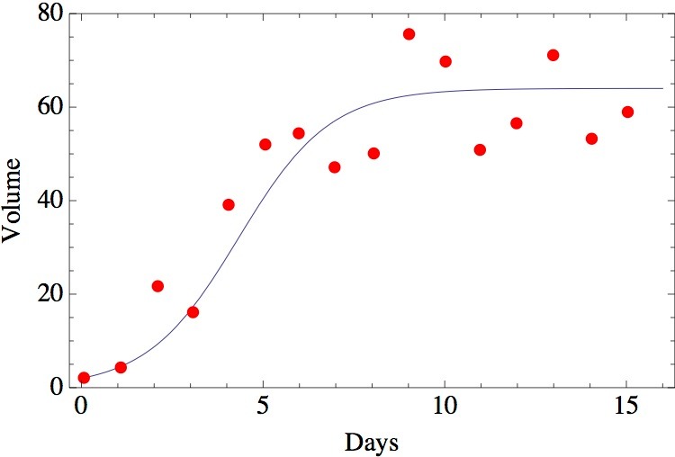
The logistic function P(t) in the above figure gets its name from the fact that it can be derived from a continuous-time model analogous to the logistic difference equation. It is called the logistic differential equation. In Chapter 7 we will explore this model in detail and we will see that is has the general form
where N is the population size and r and K are positive constants (see Equation 7.1.4 of the textbook). As will be seen in Section 7.4 of the textbook, to derive a function N(t) for the population size at time t from this model we need to integrate the reciprocal of the right-side of the above equation with respect to N. In other words, we need to integrate the function

or

Note that when r = 1 this function simplifies to

which is the function in Example 5.6.2 of the textbook.