Example 8.1.3 of the textbook and the associated BB material on this website explains how an assay called the hemaglutination inhibition (HI) assay can be used to measure the binding strength between an influenza virus and an antiserum. The BB material from Example 8.1.3 also explains how such data can then be transformed into a measure of the antigenic difference between each virus and each antiserum. Then, in Example 8.1.8 of the textbook and the associated BB material on this website, we saw how one can display such high-dimensional antigenic data in two dimensions. The figure below plots data using this method.
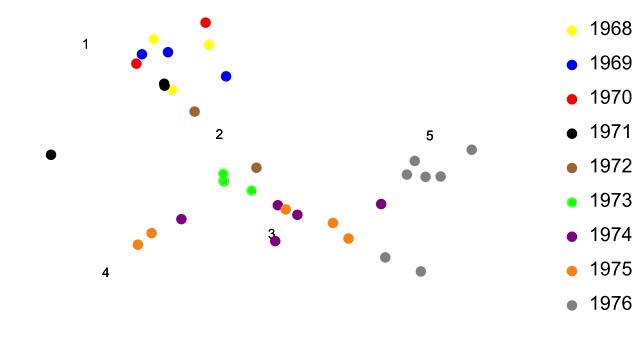
As was seen in the BB material on this website associated with Example 8.1.8 of the textbook, antigenic plots like that above are not unique. They can be translated, rotated, or reflected in the plane and the antigenic relationships among the points will remain the same. In this way, the coordinate axes of the plot are unimportant. It is only the relationships among the viruses and antisera that have meaning in the plot. Of course we are free to introduce any coordinate system that we like on plots like that above and this then allows us to treat antigenic distances and the locations of viruses algebraically. Example 8.2.3 of the textbook illustrates this idea.
References
Smith, D.J. et al. 2004. Mapping the antigenic and genetic evolution of influenza virus. Science 305: .371-376